Frequently Asked Questions (FAQ)
How do I control the way my DataFrame is displayed?
Pandas users rely on a variety of environments for using pandas: scripts, terminal, IPython qtconsole/ notebook, (IDLE, spyder, etc’). Each environment has it’s own capabilities and limitations: HTML support, horizontal scrolling, auto-detection of width/height. To appropriately address all these environments, the display behavior is controlled by several options, which you’re encouraged to tweak to suit your setup.
As of 0.12, these are the relevant options, all under the display namespace, (e.g. display.width, etc’):
- notebook_repr_html: if True, IPython frontends with HTML support will display dataframes as HTML tables when possible.
- expand_repr (default True): when the frame width cannot fit within the screen, the output will be broken into multiple pages to accomedate. This applies to textual (as opposed to HTML) display only.
- max_columns: max dataframe columns to display. a wider frame will trigger a summary view, unless expand_repr is True and HTML output is disabled.
- max_rows: max dataframe rows display. a longer frame will trigger a summary view.
- width: width of display screen in characters, used to determine the width of lines when expand_repr is active, Setting this to None will trigger auto-detection of terminal width, this only works for proper terminals, not IPython frontends such as ipnb. width is ignored in IPython notebook, since the browser provides horizontal scrolling.
IPython users can use the IPython startup file to import pandas and set these options automatically when starting up.
Adding Features to your Pandas Installation
Pandas is a powerful tool and already has a plethora of data manipulation operations implemented, most of them are very fast as well. It’s very possible however that certain functionality that would make your life easier is missing. In that case you have several options:
Open an issue on Github , explain your need and the sort of functionality you would like to see implemented.
Fork the repo, Implement the functionality yourself and open a PR on Github.
Write a method that performs the operation you are interested in and Monkey-patch the pandas class as part of your IPython profile startup or PYTHONSTARTUP file.
For example, here is an example of adding an just_foo_cols() method to the dataframe class:
In [1]: import pandas as pd

In [2]: def just_foo_cols(self):
   ...:     """Get a list of column names containing the string 'foo'
   ...:     """
   ...:     return [x for x in self.columns if 'foo' in x]
   ...:

In [3]: pd.DataFrame.just_foo_cols = just_foo_cols # monkey-patch the DataFrame class

In [4]: df = pd.DataFrame([list(range(4))], columns=["A","foo","foozball","bar"])

In [5]: df.just_foo_cols()
['foo', 'foozball']

In [6]: del pd.DataFrame.just_foo_cols # you can also remove the new method
Monkey-patching is usually frowned upon because it makes your code less portable and can cause subtle bugs in some circumstances. Monkey-patching existing methods is usually a bad idea in that respect. When used with proper care, however, it’s a very useful tool to have.
Migrating from scikits.timeseries to pandas >= 0.8.0
Starting with pandas 0.8.0, users of scikits.timeseries should have all of the features that they need to migrate their code to use pandas. Portions of the scikits.timeseries codebase for implementing calendar logic and timespan frequency conversions (but not resampling, that has all been implemented from scratch from the ground up) have been ported to the pandas codebase.
The scikits.timeseries notions of Date and DateArray are responsible for implementing calendar logic:
In [16]: dt = ts.Date('Q', '1984Q3')

# sic
In [17]: dt
Out[17]: <Q-DEC : 1984Q1>

In [18]: dt.asfreq('D', 'start')
Out[18]: <D : 01-Jan-1984>

In [19]: dt.asfreq('D', 'end')
Out[19]: <D : 31-Mar-1984>

In [20]: dt + 3
Out[20]: <Q-DEC : 1984Q4>
Date and DateArray from scikits.timeseries have been reincarnated in pandas Period and PeriodIndex:
In [7]: pnow('D')  # scikits.timeseries.now()
Period('2013-10-25', 'D')

In [8]: Period(year=2007, month=3, day=15, freq='D')
Period('2007-03-15', 'D')

In [9]: p = Period('1984Q3')

In [10]: p
Period('1984Q3', 'Q-DEC')

In [11]: p.asfreq('D', 'start')
Period('1984-07-01', 'D')

In [12]: p.asfreq('D', 'end')
Period('1984-09-30', 'D')

In [13]: (p + 3).asfreq('T') + 6 * 60 + 30
Period('1985-07-01 06:29', 'T')

In [14]: rng = period_range('1990', '2010', freq='A')

In [15]: rng

<class 'pandas.tseries.period.PeriodIndex'>
freq: A-DEC
[1990, ..., 2010]
length: 21

In [16]: rng.asfreq('B', 'end') - 3

<class 'pandas.tseries.period.PeriodIndex'>
freq: B
[1990-12-26, ..., 2010-12-28]
length: 21
| scikits.timeseries | pandas | Notes |
|---|---|---|
| Date | Period | A span of time, from yearly through to secondly |
| DateArray | PeriodIndex | An array of timespans |
| convert | resample | Frequency conversion in scikits.timeseries |
| convert_to_annual | pivot_annual | currently supports up to daily frequency, see GH736 |
PeriodIndex / DateArray properties and functions
The scikits.timeseries DateArray had a number of information properties. Here are the pandas equivalents:
| scikits.timeseries | pandas | Notes |
|---|---|---|
| get_steps | np.diff(idx.values) | |
| has_missing_dates | not idx.is_full | |
| is_full | idx.is_full | |
| is_valid | idx.is_monotonic and idx.is_unique | |
| is_chronological | is_monotonic | |
| arr.sort_chronologically() | idx.order() |
Frequency conversion
Frequency conversion is implemented using the resample method on TimeSeries and DataFrame objects (multiple time series). resample also works on panels (3D). Here is some code that resamples daily data to montly with scikits.timeseries:
In [17]: import scikits.timeseries as ts
---------------------------------------------------------------------------
ImportError                               Traceback (most recent call last)
<ipython-input-17-a44de061a6d8> in <module>()
----> 1 import scikits.timeseries as ts
ImportError: No module named scikits.timeseries

In [18]: data = ts.time_series(np.random.randn(50), start_date='Jan-2000', freq='M')
---------------------------------------------------------------------------
AttributeError                            Traceback (most recent call last)
<ipython-input-18-c16b12c482e8> in <module>()
----> 1 data = ts.time_series(np.random.randn(50), start_date='Jan-2000', freq='M')
/Users/jtratner/projects/python/pandas/pandas/core/generic.pyc in __getattr__(self, name)
   1470             return self[name]
   1471         raise AttributeError("'%s' object has no attribute '%s'" %
-> 1472                              (type(self).__name__, name))
   1473
   1474     def __setattr__(self, name, value):
AttributeError: 'Series' object has no attribute 'time_series'

In [19]: data

{'Label1': <class 'pandas.core.panel.Panel'>
Dimensions: 1 (items) x 4 (major_axis) x 3 (minor_axis)
Items axis: Item1 to Item1
Major_axis axis: 0 to 3
Minor_axis axis: 0 to 2,
 'Label2': <class 'pandas.core.panel.Panel'>
Dimensions: 1 (items) x 4 (major_axis) x 2 (minor_axis)
Items axis: Item2 to Item2
Major_axis axis: 0 to 3
Minor_axis axis: 0 to 1}

In [20]: data.convert('A', func=np.mean)
---------------------------------------------------------------------------
AttributeError                            Traceback (most recent call last)
<ipython-input-20-42ee10087ca8> in <module>()
----> 1 data.convert('A', func=np.mean)
AttributeError: 'dict' object has no attribute 'convert'
Here is the equivalent pandas code:
In [21]: rng = period_range('Jan-2000', periods=50, freq='M')

In [22]: data = Series(np.random.randn(50), index=rng)

In [23]: data

2000-01    0.469112
2000-02   -0.282863
2000-03   -1.509059
2000-04   -1.135632
2000-05    1.212112
2000-06   -0.173215
2000-07    0.119209
2000-08   -1.044236
2000-09   -0.861849
2000-10   -2.104569
2000-11   -0.494929
2000-12    1.071804
2001-01    0.721555
2001-02   -0.706771
2001-03   -1.039575
2001-04    0.271860
2001-05   -0.424972
2001-06    0.567020
2001-07    0.276232
2001-08   -1.087401
2001-09   -0.673690
2001-10    0.113648
2001-11   -1.478427
2001-12    0.524988
2002-01    0.404705
2002-02    0.577046
2002-03   -1.715002
2002-04   -1.039268
2002-05   -0.370647
2002-06   -1.157892
2002-07   -1.344312
2002-08    0.844885
2002-09    1.075770
2002-10   -0.109050
2002-11    1.643563
2002-12   -1.469388
2003-01    0.357021
2003-02   -0.674600
2003-03   -1.776904
2003-04   -0.968914
2003-05   -1.294524
2003-06    0.413738
2003-07    0.276662
2003-08   -0.472035
2003-09   -0.013960
2003-10   -0.362543
2003-11   -0.006154
2003-12   -0.923061
2004-01    0.895717
2004-02    0.805244
Freq: M, dtype: float64

In [24]: data.resample('A', how=np.mean)

2000   -0.394510
2001   -0.244628
2002   -0.221633
2003   -0.453773
2004    0.850481
Freq: A-DEC, dtype: float64
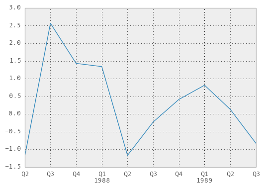
Plotting
Much of the plotting functionality of scikits.timeseries has been ported and adopted to pandas’s data structures. For example:
In [25]: rng = period_range('1987Q2', periods=10, freq='Q-DEC')

In [26]: data = Series(np.random.randn(10), index=rng)

In [27]: plt.figure(); data.plot()
<matplotlib.axes.AxesSubplot at 0x1077f3350>
Converting to and from period format
Use the to_timestamp and to_period instance methods.
Treatment of missing data
Unlike scikits.timeseries, pandas data structures are not based on NumPy’s MaskedArray object. Missing data is represented as NaN in numerical arrays and either as None or NaN in non-numerical arrays. Implementing a version of pandas’s data structures that use MaskedArray is possible but would require the involvement of a dedicated maintainer. Active pandas developers are not interested in this.
Resampling with timestamps and periods
resample has a kind argument which allows you to resample time series with a DatetimeIndex to PeriodIndex:
In [28]: rng = date_range('1/1/2000', periods=200, freq='D')

In [29]: data = Series(np.random.randn(200), index=rng)

In [30]: data[:10]

2000-01-01   -0.076467
2000-01-02   -1.187678
2000-01-03    1.130127
2000-01-04   -1.436737
2000-01-05   -1.413681
2000-01-06    1.607920
2000-01-07    1.024180
2000-01-08    0.569605
2000-01-09    0.875906
2000-01-10   -2.211372
Freq: D, dtype: float64

In [31]: data.index

<class 'pandas.tseries.index.DatetimeIndex'>
[2000-01-01 00:00:00, ..., 2000-07-18 00:00:00]
Length: 200, Freq: D, Timezone: None

In [32]: data.resample('M', kind='period')

2000-01   -0.175775
2000-02    0.094874
2000-03    0.124949
2000-04    0.066215
2000-05   -0.040364
2000-06    0.116263
2000-07   -0.263235
Freq: M, dtype: float64
Similarly, resampling from periods to timestamps is possible with an optional interval ('start' or 'end') convention:
In [33]: rng = period_range('Jan-2000', periods=50, freq='M')

In [34]: data = Series(np.random.randn(50), index=rng)

In [35]: resampled = data.resample('A', kind='timestamp', convention='end')

In [36]: resampled.index

<class 'pandas.tseries.index.DatetimeIndex'>
[2000-12-31 00:00:00, ..., 2004-12-31 00:00:00]
Length: 5, Freq: A-DEC, Timezone: None
Byte-Ordering Issues
Occasionally you may have to deal with data that were created on a machine with a different byte order than the one on which you are running Python. To deal with this issue you should convert the underlying NumPy array to the native system byte order before passing it to Series/DataFrame/Panel constructors using something similar to the following:
In [37]: x = np.array(list(range(10)), '>i4') # big endian

In [38]: newx = x.byteswap().newbyteorder() # force native byteorder

In [39]: s = Series(newx)
See the NumPy documentation on byte order for more details.
Visualizing Data in Qt applications
There is experimental support for visualizing DataFrames in PyQt4 and PySide applications. At the moment you can display and edit the values of the cells in the DataFrame. Qt will take care of displaying just the portion of the DataFrame that is currently visible and the edits will be immediately saved to the underlying DataFrame
To demonstrate this we will create a simple PySide application that will switch between two editable DataFrames. For this will use the DataFrameModel class that handles the access to the DataFrame, and the DataFrameWidget, which is just a thin layer around the QTableView.
import numpy as np
import pandas as pd
from pandas.sandbox.qtpandas import DataFrameModel, DataFrameWidget
from PySide import QtGui, QtCore

# Or if you use PyQt4:
# from PyQt4 import QtGui, QtCore

class MainWidget(QtGui.QWidget):
    def __init__(self, parent=None):
        super(MainWidget, self).__init__(parent)

        # Create two DataFrames
        self.df1 = pd.DataFrame(np.arange(9).reshape(3, 3),
                                columns=['foo', 'bar', 'baz'])
        self.df2 = pd.DataFrame({
                'int': [1, 2, 3],
                'float': [1.5, 2.5, 3.5],
                'string': ['a', 'b', 'c'],
                'nan': [np.nan, np.nan, np.nan]
            }, index=['AAA', 'BBB', 'CCC'],
            columns=['int', 'float', 'string', 'nan'])

        # Create the widget and set the first DataFrame
        self.widget = DataFrameWidget(self.df1)

        # Create the buttons for changing DataFrames
        self.button_first = QtGui.QPushButton('First')
        self.button_first.clicked.connect(self.on_first_click)
        self.button_second = QtGui.QPushButton('Second')
        self.button_second.clicked.connect(self.on_second_click)

        # Set the layout
        vbox = QtGui.QVBoxLayout()
        vbox.addWidget(self.widget)
        hbox = QtGui.QHBoxLayout()
        hbox.addWidget(self.button_first)
        hbox.addWidget(self.button_second)
        vbox.addLayout(hbox)
        self.setLayout(vbox)

    def on_first_click(self):
        '''Sets the first DataFrame'''
        self.widget.setDataFrame(self.df1)

    def on_second_click(self):
        '''Sets the second DataFrame'''
        self.widget.setDataFrame(self.df2)

if __name__ == '__main__':
    import sys

    # Initialize the application
    app = QtGui.QApplication(sys.argv)
    mw = MainWidget()
    mw.show()
    app.exec_()